Trying to keep people engaged in my fantasy football league is an ongoing struggle. Because of this I started a ghost blog on for my league to have some weekly posts go out to generate some engagement from the other league members. I also did not want to spend a lot of time writing posts every week so I figured automating the data gathering aspect and making a few predictions using ESPN's API (which is undocumented for whatever reason) would be a good way to go.
ESPN API
As I mentioned before ESPN fantasy does have a fantasy football API, but it is not really documented and changes quite often (just a few days ago they added pagination to their results breaking a bunch of code). However as of this writing (2/10/2021) the following endpoint works and is what I used.
leagueID=LEAGUEID
w=WEEKNUMBER
scoreboard=requests.get('http://fantasy.espn.com/apis/v3/games/ffl/seasons/2020/' \
'segments/0/leagues/{}?view=mBoxscore&scoringPeriodId={}&matchupPeriodId={}'.format(leagueID,w,w))
If we set up the scoringPeriodID and the matchupPeriodID as the same we can pull the scores for that week as well as the projections.
The values returned provide us with both the team names, the actual score, the projected score and per player statistics. There are also other endpoints, the most useful which is the per player projections.
import requests

url = "https://fantasy.espn.com/apis/v3/games/ffl/ \
seasons/2020/segments/0/leagues/{}?view=kona_player_info".format(leagueID)

headers = {
  'X-Fantasy-Filter': '{"players": \
    {"filterStatus":\
      {"value":["FREEAGENT","WAIVERS"]},\
      "filterSlotIds":{"value":[0,1,2,3,4,5,6,7,8,9,10,11,12,13,14,15,16,17,18,19,23,24]},\
      "filterRanksForScoringPeriodIds":{"value":[2]},\
      "sortPercOwned":{"sortAsc":false,"sortPriority":1},\
      "sortDraftRanks":{"sortPriority":100,"sortAsc":true,"value":"STANDARD"},\
      "filterRanksForRankTypes":{"value":["PPR"]},\
      "filterRanksForSlotIds":{"value":[0,2,4,6,17,16]},\
      "filterStatsForTopScoringPeriodIds":{"value":2,\
                    "additionalValue":["002020","102020","002019","1120202","022020"]}}}',\
  'Cookie': 'region=unknown; _dcf=1'
}

response = requests.request("GET", url, headers=headers)
I don't really use this endpoint for the Summary and Preview posts, but it is interesting for making my own projections and similar. Using the Dev Console on any browser you can figure out the necessary values for the X-Fantasy-Filter dictionary and they are pretty self-explanatory.
Summary Post
The first post I wanted to automate was the summary post for the previous weeks matchups. For each match I need to pull the scores and for a fun stat also look at all the possible team combinations for each roster and figures out if the player actually picked a decent team or if he had done better randomly selecting his team.
First we generate a couple of dictionaries to help with generating the post.
sc_data=scoreboard.json()

#Position ID to description
pos_dict={0:'QB',2:'RB',4:'WR',6:'TE',23:'FLEX',16:'D/ST',17:'K',20:'BNCK'}

#Allowable number of players in position per active roster
Rs={0:1,2:2,4:2,6:1,23:1,16:1,17:1}

#Team names to team id
team_map={itm['id']:itm['location']+' '+itm['nickname'] for itm in sc_data['teams']}
iteam_map = {v: k for k, v in team_map.items()}

#My league has three dvisions
divs={0:'East',1:'West',2:'Mid'}

#What division each team is in
team_div={x['id']:divs.get(x['divisionId']) for x in sc_data['teams']}
Now that we have the dictionary we will get each team, their scores, and all the possible team combinations along with their possible scores.
#Dictionary to hold each teams information
gscores={}

#The match id for that week
gno=1
#Iterate over each game in the schedule
for s in sc_data['schedule']:
    if s['matchupPeriodId']==w:
        print('---------')
        print("home: {} away {}".format(s['home']['teamId'],s['away']['teamId']))
        print('---------')
        tdict={}
        #Iterate over the home and away teams
        for ttype in ['home','away']:

            team=s[ttype]
            print(ttype.upper())
            #Store both the team roster and and the active roster
            aroster=team['rosterForMatchupPeriod']
            roster=team['rosterForCurrentScoringPeriod']
            #Empty array for lineup
            lp=[]
            for e in roster['entries']:
                pscore=e['playerPoolEntry']['appliedStatTotal']
                pfname=e['playerPoolEntry']['player']['fullName']
                pslots=e['playerPoolEntry']['player']['eligibleSlots']
                pslot=e['lineupSlotId']
                print("{:.2f} {} Slot:{}".format(pscore,pfname,pslot),pslots)
                lp.append([pscore,pfname,pslot,pslots])

            #Create a dataframe holding each player, the slot they are in,
            # and the possible positions they could play in
            lpd=pd.DataFrame(lp,columns=['Score','Name','Slot','Slots'])
            lpd['SlotPos']=lpd.Slot.map(pos_dict)
            lpd.SlotPos.fillna('Unknown',inplace=True)
            posln={}

            for k in Rs:
                posln[k]=lpd[lpd.Slots.apply(lambda x:k in x)].index.values

            #Tarr store the index of lpd based on the quantities stored in the Rs
            #dictionary previously stored
            tarr=[]
            for i,k in Rs.items():
                for ii in range(0,k):
                    tarr.append(list(posln[i]))

            #Create an empty array that contain each possible lineup's scores
            lpscore=[]

            #Generate each combination based on the arrays in tarr
            #Keep only the ones that have 9 distinct players
            for lpos in itertools.product(*tarr):
                if len(set(lpos))==9:
                    lpscore.append(lpd.loc[list(lpos)].Score.sum())

            tdict[ttype]={'score':roster['appliedStatTotal'],'roster':lpd,'teamid':team['teamId'],'pos':lpscore}
        gscores[gno]=tdict
        gno=gno+1
For each team roster our lpd will look like this (Unknown is used for the IR spots)
| Score | Name | Slot | Slots | SlotPos | |
|---|---|---|---|---|---|
| 0 | 0 | Miles Sanders | 21 | [2, 3, 23, 7, 20, 21] | Unknown |
| 1 | 14 | Travis Kelce | 6 | [5, 6, 23, 7, 20, 21] | TE |
| 2 | 0 | Courtland Sutton | 21 | [3, 4, 5, 23, 7, 20, 21] | Unknown |
| 3 | 6.4 | A.J. Brown | 4 | [3, 4, 5, 23, 7, 20, 21] | WR |
| 4 | 2.4 | Leonard Fournette | 2 | [2, 3, 23, 7, 20, 21] | RB |
| 5 | 5.6 | Le'Veon Bell | 23 | [2, 3, 23, 7, 20, 21] | FLEX |
| 6 | 6.7 | DeVante Parker | 20 | [3, 4, 5, 23, 7, 20, 21] | BNCK |
| 7 | 10.5 | Julian Edelman | 20 | [3, 4, 5, 23, 7, 20, 21] | BNCK |
| 8 | 28.18 | Josh Allen | 0 | [0, 7, 20, 21] | QB |
| 9 | 22.4 | Robby Anderson | 20 | [3, 4, 5, 23, 7, 20, 21] | BNCK |
| 10 | 23.3 | Nyheim Hines | 20 | [2, 3, 23, 7, 20, 21] | BNCK |
| 11 | 6.4 | Boston Scott | 2 | [2, 3, 23, 7, 20, 21] | RB |
| 12 | 6.5 | Steven Sims Jr. | 20 | [3, 4, 5, 23, 7, 20, 21] | BNCK |
| 13 | 17 | Saints D/ST | 16 | [16, 20, 21] | D/ST |
| 14 | 22.06 | Ben Roethlisberger | 20 | [0, 7, 20, 21] | BNCK |
| 15 | 7 | Rodrigo Blankenship | 17 | [25, 17, 20, 21] | K |
| 16 | 4.5 | Mike Gesicki | 20 | [5, 6, 23, 7, 20, 21] | BNCK |
| 17 | 4.9 | Tim Patrick | 4 | [3, 4, 5, 23, 7, 20, 21] | WR |
and our tarr looks like this
[[8, 14],
 [0, 4, 5, 10, 11],
 [0, 4, 5, 10, 11],
 [2, 3, 6, 7, 9, 12, 17],
 [2, 3, 6, 7, 9, 12, 17],
 [1, 16],
 [0, 1, 2, 3, 4, 5, 6, 7, 9, 10, 11, 12, 16, 17],
 [13],
 [15]]
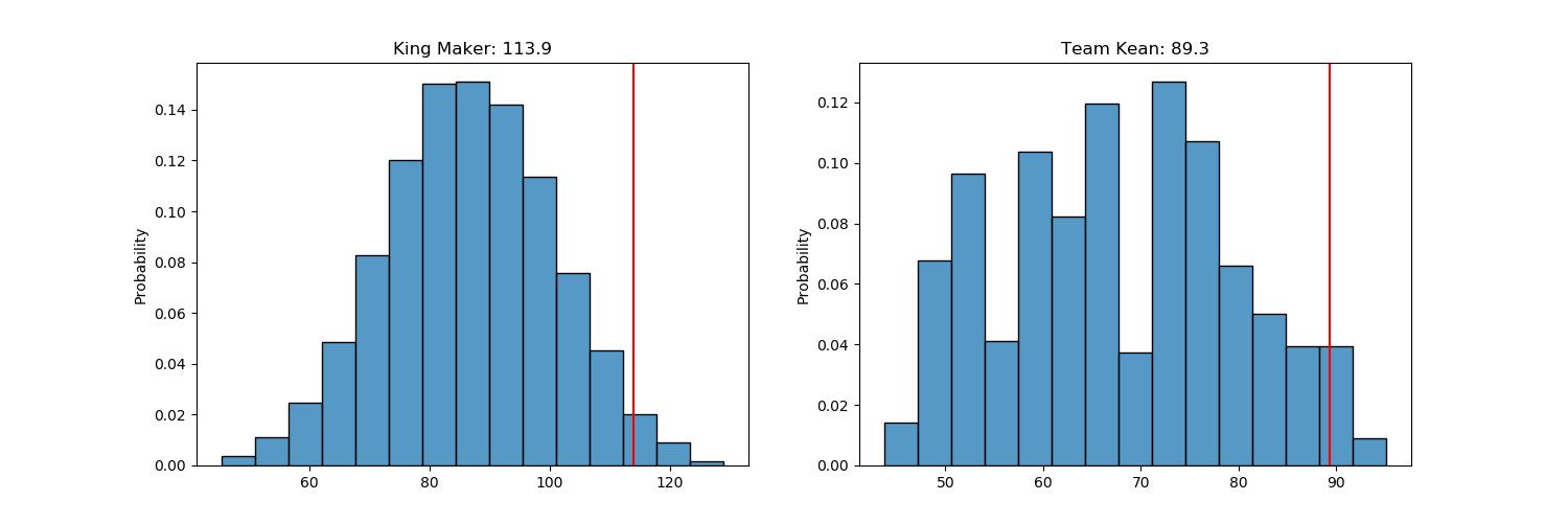
A quick check makes sure that it matches what we would think. Since we have all the information available we can generate histograms that will show us the performance of each lineup.
heading=[]
#Seaborn setup
sns.set_theme(style="ticks",font_scale=1.2, color_codes=True)
tds=pd.DataFrame([],columns=['team'])
#Make a nice datframe with all the teams (for our box plot)
all_rosters=pd.DataFrame([])
for i,g in gscores.items():
    print('GAME '+str(i))
    home=team_map.get(g['home']['teamid'])
    away=team_map.get(g['away']['teamid'])
    home_score=g['home']['score']
    away_score=g['away']['score']
    ##WE create a sybtutke
    heading.append('{}: {:.1f} vs {}: {:.1f}'.format(home,home_score,away,away_score))
    print('{}: {:.1f} vs {}: {:.1f}'.format(home,home_score,away,away_score))
    f, (ax1, ax2) = plt.subplots(1, 2, sharey=False,figsize=(15,5))

    #pd.Series(g['home']['pos']).hist(ax=ax1,bins=15, grid=False,facecolor='b',edgecolor='k')
    sns.histplot(g['home']['pos'],ax=ax1,bins=15,stat="probability")
    ax1.axvline(g['home']['score'],color='r')
    ax1.set_title('{}:{:.1f}'.format(home,home_score))

    #pd.Series(g['away']['pos']).hist(ax=ax2,bins=15, grid=False,facecolor='b',edgecolor='k')
    sns.histplot(g['away']['pos'],ax=ax2,bins=15,stat="probability")
    ax2.axvline(g['away']['score'],color='r')
    ax2.set_title('{}: {:.1f}'.format(away,away_score))

    td=pd.DataFrame(g['home']['pos'],columns=['score'])
    td.insert(column='team',value=home,loc=0)
    td.insert(column='sc',value=home_score,loc=0)
    tds=tds.append(td)
    all_rosters=all_rosters.append(g['home']['roster'])

    td=pd.DataFrame(g['away']['pos'],columns=['score'])
    td.insert(column='team',value=away,loc=0)
    td.insert(column='sc',value=away_score,loc=0)
    tds=tds.append(td)
    plt.savefig('Week{}/g{}_prob.png'.format(w,i))
    all_rosters=all_rosters.append(g['away']['roster'])
So we will end up with each matchup histogram. For example:

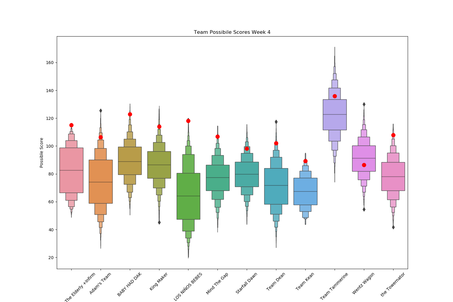
Finally for a overall view of each teams performance we can do the following:
fb,axbp = plt.subplots(figsize=(15,10))

sns.boxenplot(x="team", y='score', data=tds, ax=axbp)
sns.stripplot(data=tds[['team','sc']].drop_duplicates(), x="team", y="sc",color='r',jitter=0,size=10)
axbp.tick_params(axis='x', labelrotation=45)
axbp.set_title('Team Possibile Scores Week 1');
axbp.set(xlabel='Team', ylabel='Possible Score');
plt.savefig('Week{}/overall_prob.png'.format(w))
Which gives us the following plot, with the red dot representing the actual team score

Finally we calculate some fun stats (team with the top best possible score and team with the worst best possible score. We also calculate the league MVP and LVP (in terms of points scored versus other players in the position).
bsc=tds.groupby('team').max()
bsc.columns=['Actual Score','Best Possible Score']
bsc.index.name=''
bmax=bsc.idxmax().to_frame()
bmin=bsc.idxmin().to_frame()

perf=[]
for gname, gp in all_rosters[['Name','Score','SlotPos']][~all_rosters['SlotPos'].isin(['Unknown','BNCK'])].groupby('SlotPos'):
    sc=StandardScaler()
    gp=gp.set_index('Name')
    xs=sc.fit_transform(gp['Score'].values.reshape(-1, 1))
    gp['Scale']=xs
    pmin=gp.loc[gp.Score.idxmin()]
    pmax=gp.loc[gp.Score.idxmax()]
    perf.append([pmax.name,pmin.name,pmax.Scale,pmin.Scale])
perfdf=pd.DataFrame(perf,columns=['Max_Name','Min_Name','MaxN','MinN'])
LVP=perfdf.loc[perfdf.MinN.idxmin].Min_Name
MVP=perfdf.loc[perfdf.MaxN.idxmax].Max_Name
I also added a random quote as a subheading for the post
f = open('quotes.txt', 'r')
txt = f.read()
lines = txt.split('\n.\n')
rand=random.choice(lines)
Finally this can the moved to a markdown file that I can copy paste into ghost and then upload each plot as necessary.
filename='Week{}/stat_post.md'.format(w)
with open(filename, 'w', encoding='utf-8') as f:
    f.write("# Week {} Stats \n".format(w))
    f.write("> {}  \n".format(rand))
    f.write('## Team Performance \n')
    f.write('Team with the highest score: {}  \n'.format(bmax.loc['Actual Score'][0]))
    f.write('Team with the highest best score: {}  \n'.format(bmax.loc['Best Possible Score'][0]))
    f.write('Team with the lowest score: {}  \n'.format(bmin.loc['Actual Score'][0]))
    f.write('Team with the lowest best score: {}  \n\n'.format(bmin.loc['Best Possible Score'][0]))
    f.write(bsc.to_markdown())
    f.write('\n\n')
    f.write('Week {} MVP: {}  \n'.format(w,MVP))
    f.write('Week {} LVP: {}  \n'.format(w,LVP))
    for h in heading:
        f.write('## {} \n'.format(h))
    f.write(' \n')
    f.write('## Overall Team Performance \n')
And that is it. After they get imported into ghost I go ahead and write whatever blurb I want under each teams heading. It works pretty well and saves me a bunch of time. I have also modified this code to run as a DAG on airflow.
Jupyter Notebooks found here

