

Way back in 2013 when I was a grad student at Marquette the majority of my research was in developing optimization routines to design passive flexible components to handle robotic assembly.
I thought it would be fun to revisit some of the work I did and see if what it would look like with 10 years of improvement in opensource programs available for optimization.
When I first worked on this most of the work was done with Matlab and its excellent optimization toolbox, with some additional programs written in C++ to improve technology. Some of the optimizations took so long and I was looking at so many variations that it ended up having to be modified to be distributed onto a Condor ( Now HTCondor) cluster at Marquette.
The first step in the design task is to identify how two parts can contact and of those parts how many of them can actually occur within the bounds of our robot.
Problem Setup
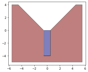
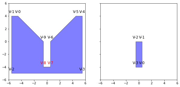
The basic setup is to define a set of two objects A and B. Object A is fixed and has a bit of an incline to assist with assembly (basically this is because you need to be able to direct the force towards proper assembly). Object B is held by the manipulator of a robot.
The robot assembly is setup within the bounds:
INIT_MAX_THETA=np.pi/36
INIT_MIN_THETA=-np.pi/36
INIT_MAX_X=1.87
INIT_MAX_Y=24.5
INIT_MIN_X=-1.87
INIT_MIN_Y=0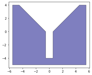
Because we are going to be doing a lot of transformation and vector calculations we first need to define our objects in Python. We will also take advantage of the shapely to handle some of our geometric evaluations.
VertA=np.array([
[-5.55, 4],
[-5.55, -5],
[5.55, -5],
[5.55, 4 ],
[4.55, 4],
[0.55, 0],
[0.55, -4],
[-0.55, -4],
[-0.55, 0],
[-4.55, 4 ]
])
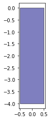
VertB=np.array([
[0.5, -4],
[-0.5, -4],
[-0.5, 0],
[0.5, 0],
])
We are using numpy arrays because we are doing vector math and regular lists wont work with that.
We need to prepare our objects for the evaluations so we define a function to do so.
from shapely.geometry import Polygon, LineString, LinearRing

def prepare_object(Vert: list, Verbose=False) -> list:
  '''
  Function taks an list of vertices
  Returns and object dictionary with geometric properties.
  '''
  #Check that object is defined as ccw
  LRObjB=LinearRing(Vert)
  if LRObjB.is_ccw is not True:
    Vert=[x for x in reversed(Vert)]
  Lines=[]
  Vectors=[]
  VectorsNorm=[]
  Edges=[]
  Verts2=[]

  # For each create an edge, a shapely line and also due to how we want iterate
  # rework our Vertices to mantain the shape. Normalize our Vectors
  for i in range(len(Vert)):
    Edge=[Vert[i-1],Vert[i]]
    Edges.append(Edge)
    Line=LineString([Vert[i-1],Vert[i]])
    Lines.append(Line)
    Verts2.append(Vert[i-1])
    Vector=np.array(Vert[i-1])-np.array(Vert[i])
    Vectors.append(Vector)
    VectorNorm = Vector/np.linalg.norm(Vector)
    VectorsNorm.append(VectorNorm)


  # Get the vectors of each 2D object.Super easy for 2D
  Normals=[]
  for V in VectorsNorm:
    Norm=np.array([-V[1],V[0]])
    Normals.append(Norm)

  if Verbose:
    print("Edges")
    print('\n'.join('{}: {}'.format(*k) for k in enumerate(Edges)))

    print("Vertices")
    print('\n'.join('{}: {}'.format(*k) for k in enumerate(Verts2)))

    print("Normals")
    print('\n'.join('{}: {}'.format(*k) for k in enumerate(Normals)))

    print("Vectors")
    print('\n'.join('{}: {}'.format(*k) for k in enumerate(Vectors)))
    print("Vectors Normalized")
    print('\n'.join('{}: {}'.format(*k) for k in enumerate(VectorsNorm)))
  Obj={}
  Obj['Vertices']=np.asarray(Verts2)
  Obj['Edges']=Edges
  Obj['Lines']=Lines
  Obj['Vectors']=Vectors
  Obj['VectorsNorm']=VectorsNorm
  Obj['Normals']=Normals
  return Obj
This returns an object dictionary (which really should be a class but I am a bit lazy). That has information regarding the Vertices, Edges, Lines, Vectors and Normals of the object. We also use the shapely class LinearRing to determine if our object is ccw or not. We want to keep this consistent so we can do our cross products the same way.
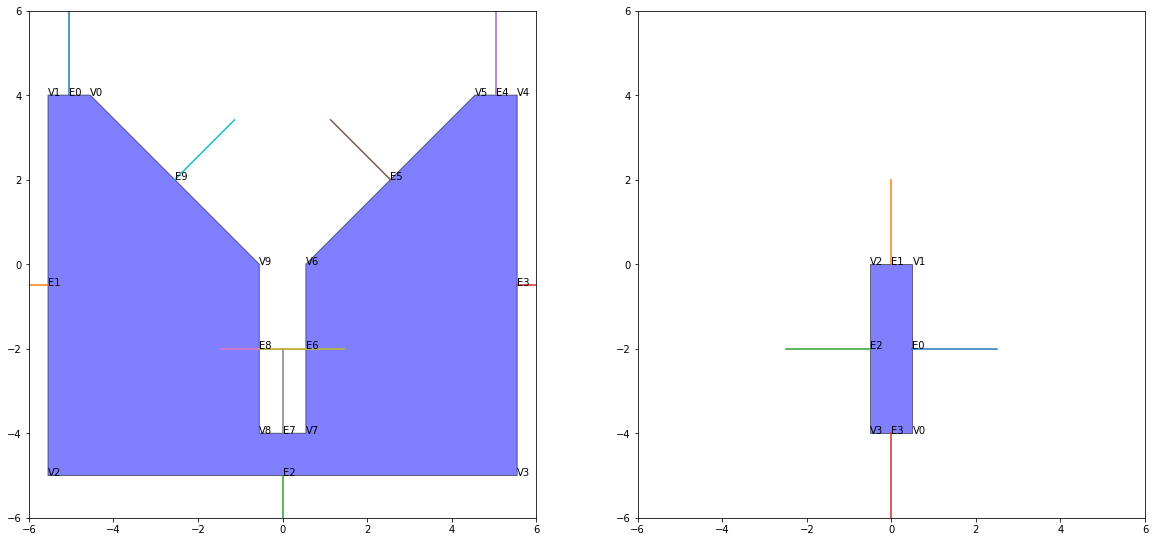
We can check how our objects look. Since this is a simplification of a 3d problem our face normals are just the line normals with z=0
Concave Points
If you spend any time looking at identifying contact between objects (or in general dealing with objects in space). You don't really want to deal with concave objects, and if you do you want to make sure you identify which vertices are causing it. For Obj A, it is clear it is concave. We identify this by taking a dot product and using the adjacent defining vectors.
def get_concave(ObjData: list) -> list:
    """
    Function takes an Object dictionary and returns a list of concave vertices
    for each one by looking at the attached vertices
    returns a lsit with the values
    """
    ConcaveList=[]
    for i in range(len(ObjData['Vertices'])):
        x1=np.take(ObjData['Vertices'],i, axis=0, mode='wrap')

        be1=np.take(ObjData['Normals'],i-1, axis=0, mode='wrap')
        be2=np.take(ObjData['Normals'],i, axis=0, mode='wrap')

        be1=np.append(be1,0)
        be2=np.append(be2,0)

        v=np.cross(be1,be2)

        v0=np.append(x1,0)
        v2=np.append(x1,-1)

        res=np.dot(-v, (v2- v0))

        ConcaveList.append(res)
    return ConcaveList
If the value is negative then the vertex is concave.
Identifying primitive Contact States
Now we can get started with identifying the contact states. We want to reduce the time it takes so first we utilize our bounds and list of concave vertices to create a list of primitive contact states that we are going to look at feasibility for.
This is a lengthy process so for this post I will only look at what we call Vertex-Edge contacts (V-E going forward).
First we want to remove all of the contacts that involve the concave vertices, since for this problem they would be considered correct assembly.
Then we want to look at how much we would have to rotate to actually have contact. So for example we would not be able to contact Obj A: V9 to Obj B: E0 since that would require fully fliping the part.
def get_angle_vector(a: npt.DTypeLike, b: npt.DTypeLike) -> float:
    '''
    Function to determine the angle bewteen two vectors
    Returns the angle in radians
    '''
    a1=np.arccos(a[0]/np.linalg.norm(a))
    a2=np.arccos(b[0]/np.linalg.norm(b))

    if a[1]<0:
        a1=-a1

    if b[1]<0:
        a2=-a2

    angle=a1-a2

    if angle>np.pi:
        angle=angle-2*np.pi
    elif angle<=-np.pi:
        angle=angle+2*np.pi

    return angle

def VE_feas(Angle_a: float, Angle_b: float) -> list[float, float, bool]:
    '''
    Function to determine if a rotation angle is feasable
    returns the minimum, maxium and feasability of the operation
    '''
    a_max=np.max([Angle_a, Angle_b])
    a_min=np.min([Angle_a, Angle_b])

    if a_max-a_min > np.pi:
        temp=a_max
        a_max=a_min+2*np.pi
        a_min=temp

    if a_max<INIT_MIN_THETA or a_min>INIT_MAX_THETA:
        feas=False
    else:
        feas=True

    return a_min, a_max, feas

# Initialize an empty contact state list
ContactStates=[]

for iA, (vA, cl) in enumerate(zip(ObjA['Vertices'], ObjA['Concave'])):
    # If contact doesnt include a concave vertex
    if cl>0:
        Ea=ObjA['Normals'][iA]
        Eb=ObjA['Normals'][iA-1]

        for iB, NB in enumerate(ObjB['Normals']):
            temp=-NB
            Angle_a=get_angle_vector(Ea, temp)
            Angle_b=get_angle_vector(Eb, temp)
            a_min, a_max, feas=VE_feas(Angle_a, Angle_b)
            if feas:
                print('V {}, E{}, Angle_Min {}, Angle_Max {}'.format(iA, iB,
                math.degrees(a_min), math.degrees(a_max)))
                cs={'Type':'V-E',
                    'ID':'V{}-E{}'.format(iA, iB),
                    'ElementA':vA,
                    'ElementB':ObjB['Edges'][iB],
                    'a_min':a_min,
                    'a_max':a_max}
                ContactStates.append(cs)
This results in the following possible contact states
V 0, E3, Angle_Min -45.0, Angle_Max 0.0
V 1, E0, Angle_Min -90.0, Angle_Max 0.0
V 1, E3, Angle_Min 0.0, Angle_Max 90.0
V 2, E0, Angle_Min 0.0, Angle_Max 90.0
V 2, E1, Angle_Min -90.0, Angle_Max 0.0
V 3, E1, Angle_Min 0.0, Angle_Max 90.0
V 3, E2, Angle_Min -90.0, Angle_Max 0.0
V 4, E2, Angle_Min 0.0, Angle_Max 90.0
V 4, E3, Angle_Min -90.0, Angle_Max 0.0
V 5, E3, Angle_Min 0.0, Angle_Max 45.0
V 6, E0, Angle_Min -45.0, Angle_Max 0.0
V 9, E2, Angle_Min 0.0, Angle_Max 45.0
Feasibility of Contact States
Now that we have the possible contacts we need to actually determine if they are possible within the bounds we previously defined. In order to do so the approach is to generate an optimization to look at the possible configuration space and evaluate if that constitutes an valid assembly (for example V0-E4 which is outside the bounds of the robot).
Getting the distance between Vertex and Edge
There are two main values that determine if a contact state can occur.
- The distance between the object features
- The penetration between the objects
The first value we look at is looking at the distance between the object features. For a Vertex Edge contact this is given to us by two values. The distance from the point to the line h1 and the distance along the line vector from a point projected onto it to the boundary points that define the segment h2.
For h1 we just use the 3d vector formula. This means we take the cross product for the two vectors and divide by the normal length between the boundary points (A, B).
\[ v_1=P-A \]
\[v_2=B-A \]
\[ h1 = \frac{ v_2 \times v_1}{A-B} \]
So we can use the following code to institute these measures
def mu_f(x: float) -> float:
  """
  Return the absolute value of x as lonf as it is les than 0 (-1E-3 to help with calculations)
  Returns the absolute value or zero
  """
  if x < -1E-3:
      val = abs(x)
  else:
      val = 0
  return val

def get_h1(P: npt.DTypeLike,A: npt.DTypeLike ,B: npt.DTypeLike, verbose=False) -> list[float, np.array, float]:
  """
  Return the distance from the point to the line
  by taking the cross product of the vector from the pt to a
  line segment boundary
  Return the distance and the two vectors
  """
  v1=P-A
  v2=B-A
  # Make them be a three vector for sanity on cross products
  v1=np.append(v1,0)
  v2=np.append(v2,0)
  # Get the length of the vector from A to B
  normalLength=np.linalg.norm(A-B)

  # Get the crossproduct and divide by our normal.
  h1=abs(np.cross(v1,v2))/normalLength
  h1_2 = abs((P[0]-A[0])*(B[1]-A[1])-(P[1]-A[1])*(B[0]-A[0]))/normalLength
  if verbose:
    print('h1: {} h1_2: {}'.format(h1, h1_2))
  # Return just the z component
  if h1[-1]<=thresh:
    res=0.0
  else:
    res=h1[-1]
  return res, v1, v2
We also want to determine the distance from the projected point. If the perpendicular distance form the point lands inside the bounded segment that distance is zero, if not we get the measurement along the x component.
\[ v_{1c} \frac{(v_1 \times v_w) \times (v_2)}{v_2 \dot v_2} \]
\[ P_{p} = P + v_{1c} \]
If \(A_x -B_x == 0) \) then:
\[ \alpha = \frac{P_{py} - A_y)|A-B|}{B_y-A_y} \]
else
\[ \alpha = \frac{P_{px} - A_x)|A-B|}{B_x-A_x} \]
Then the value of h2 is going to be
\[ h_2 = \mu(\alpha)+\mu(|B-A|-\alpha) \]
Where \( \mu \) is just a function that returns \( x \} if the \( x \) negative else it returns \( 0 \).
The python code will look as follows:
def get_h2(P: npt.DTypeLike, A: npt.DTypeLike, B: npt.DTypeLike) -> tuple[float, np.array, np.array]:
  """
  Return the distance from a projected point on to the line defined by A,B
  to the boundary of the line defined by A,B. It returns 0 if the point is in the line.
  Return the mesure and the projection vector
  """
  v1=P-A
  v2=B-A

  # Make them be a three vector for sanity on cross products
  v1=np.append(v1,0)
  v2=np.append(v2,0)

  # Get the length of the vector from A to B
  normalLength=np.linalg.norm(A-B)

  #Get a vector that projects the point perpedicular to our infinate line.
  temp=np.cross(v1,v2)
  v1c=np.cross(temp,v2)/np.dot(v2,v2)

  #Project the point
  Pp=P+v1c[:2]

  # Obtain alpha as the distance from projected point to line segment
  if A[0]-B[0]==0:
    alpha=((Pp[1]-A[1])*normalLength)/(B[1]-A[1])
  else:
    alpha=((Pp[0]-A[0])*normalLength)/(B[0]-A[0])

  # Set it to zero if the projected is on the line segment
  h2=mu_f(alpha)+mu_f(normalLength-alpha)
  if h2<thresh:
    h2=0
  return h2, v1c, Pp
So with the value h1+h2 we have a measure of the distance between the features (V-E)
Getting the Penetration
Ok so now we need to determine the amount of penetration that is occurring between the parts. This is a problem that is quite common in video game design, however most algorithms are more concerned with determining if contact occurs not so much the measure of the interference.
The first step is to triangulate our objects into smaller triangles. This is done because as stated before concave objects don't play nice with most methods. To do so we use the sect package.
from ground.base import get_context
from sect.triangulation import Triangulation

def constrained_triangulation(Obj: dict) -> list:
  """
  Takes an object dictionary and triangulates
  Returns the suboject array
  """
  context= get_context()
  Contour, Point = context.contour_cls, context.point_cls
  PolygonSect = context.polygon_cls

  objContour = Contour([Point(vct[0], vct[1]) for vct in Obj['Vertices']])
  sect_objcontour = PolygonSect(objContour,[])

  subObjs=Triangulation.constrained_delaunay(sect_objcontour, context=context).triangles()
  subObjsV = [[(vert.x, vert.y) for vert in subObj.vertices] for subObj in subObjs]

  return subObjsV
This results in all our objects being broken up into smaller sub-objects.
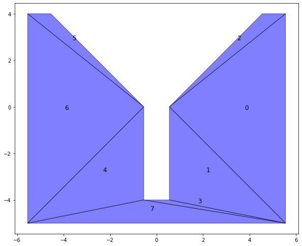
We now prepare the sub-objects as we did previously.
# We prepare each of these subobjects as we initially did for the
subObjsA=[prepare_object(subObjs) for subObjs in subObjsA]
subObjsB=[prepare_object(subObjs) for subObjs in subObjsB]
Growth Distance GJK-EPA like measure calculation
In order to get a measure of the penetration we are going to use the growth distance as outline here. It operates similarly to the GJK-EPA algorithm. However in this case we are basically identifying the point at which the expansion of the the polygons by a given factor results in interaction. There a couple more complex point in the algorithm but I recommend reading the paper to understand it. It ends up such that values less that:
- Values 0<x<1 are penetration
- x=1 contact
- x>1 expansion
In order to do so we need to determine what a stationary point that will stay inside the object when in motion. Or in simpler terms for us, one that we can uniformly scale around. Thankfully for us, the centroid of a triangle is guaranteed to have that property.
We also need to select an arbitrary point within the each face that forms the object, or for the 2D case the edges. We take a simple approach and just select the end point.
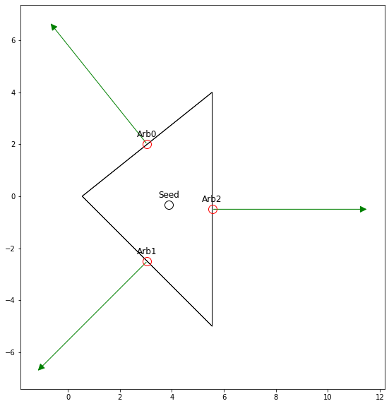
What we want to do is solve the set of equations formed by the normals for the factor that results in contact \( x=1 \).
This is a well established problem that we can solve using scipy.optimize.linprog , since its a linear objective function subject to inequality constraints of the form.
\[ min_x c^Tx \]
\[ \text{such that} \]
\[ A_{ub} \le b_{ub} \]
\[ l \le x \le u \]
In our case \( A_{ub} \) is defined by the normals \( N \) and \( -(arb_{if} - seed_{if}) \times N_{if} \) and \( b_{ub} \) is \( seed_if \times N_{if} \). Where \( if \) refers to pt/vector \( i \) defined in the frame \( f \) of the unmoveble object (in our case A). We also define an inequality such that \( -x_4 < 0 \).
The code to calculate this is as follows:
# Now wrap the whole calculation within a function

def growth_distance(subObjA, subObjB, conf):
  gdObjA = subObjA

  gdObjB = subObjB

  gdNormalsA = gdObjA['Normals']
  gdNormalsB = gdObjB['Normals']

  gdVertA = gdObjA['Vertices']
  gdVertB = gdObjB['Vertices']

  gdSeedA = gdObjA['Seed']
  gdSeedB = gdObjB['Seed']

  gdArbA = gdObjA['Arb']
  gdArbB = gdObjB['Arb']

  gdSeedBwrtA = transfer_pt(gdSeedB, conf)
  gdNormalsBwrtA = [transfer_vector(nrm, conf) for nrm in gdNormalsB]
  gdArbBwrtA = [transfer_pt(nrm, conf) for nrm in gdArbB]
  gdVertBwrtA = [transfer_pt(vert, conf) for vert in gdVertB]

  #Since we triangulated we know this is three. But for generalization we make sure
  FaceNumA = len(gdVertA)
  FaceNumB = len(gdVertB)


  #Initial Guesses for our GD and combine into the right shape
  GD = 1.0

  # Number of constraints we need
  ConNum = FaceNumA+FaceNumB+1

  # Our Object Coefficients we only need the growth function
  objCoeff = np.array([0, 0, 0, 1])

  # Right side of the inequality constraint
  conB = []
  conCoeff = []

  for arb, Nrm in zip(gdArbA, gdNormalsA):
    arb_a = np.append(arb, 0)
    nrm_a = np.append(Nrm, 0)
    seed_a = np.append(gdSeedA, 0)
    temp = -np.dot(arb_a-seed_a, nrm_a)
    conCoeff.append([nrm_a[0], nrm_a[1], nrm_a[2], temp])
    conB.append(np.dot(seed_a, nrm_a))

  for arb, Nrm in zip(gdArbBwrtA, gdNormalsBwrtA):
    arb_b = np.append(arb, 0)
    nrm_b = np.append(Nrm, 0)
    seed_b = np.append(gdSeedBwrtA, 0)
    temp = -np.dot(arb_b-seed_b, nrm_b)
    conCoeff.append([nrm_b[0], nrm_b[1], nrm_b[2], temp])
    conB.append(np.dot(seed_b, nrm_b))

  conCoeff.append([0, 0, 0, -1])
  conB.append(0)

  bounds = [(None, None) for x in range(1, 4+1)]

  res = linprog(np.array(objCoeff), A_ub=np.matrix(conCoeff),
                b_ub=np.array(conB), bounds=bounds)

  temp = np.dot(res.x, objCoeff)

  if temp <= 1-1e-4:
    gdDistance = 1-temp
  else:
    gdDistance = 0

  fscale = temp

  res_lat = []


  for lbl, mat in zip(['Obj', 'A_{{ub}}', 'B_{{ub}}'], [np.matrix(objCoeff).T, np.matrix(conCoeff), np.matrix(conB).T]):

      lat_str = '\\begin{{equation*}} {}={} \end{{equation*}}'.format(
          lbl, bmatrix(mat))
      res_lat.append(lat_str)

  return gdDistance, res, res_lat
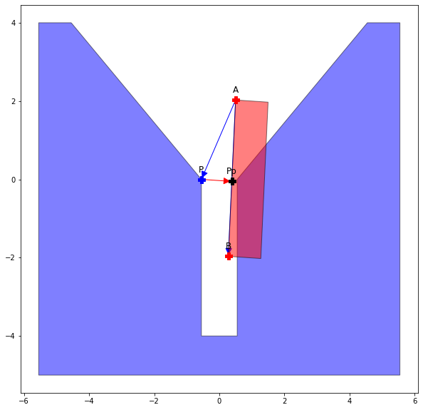
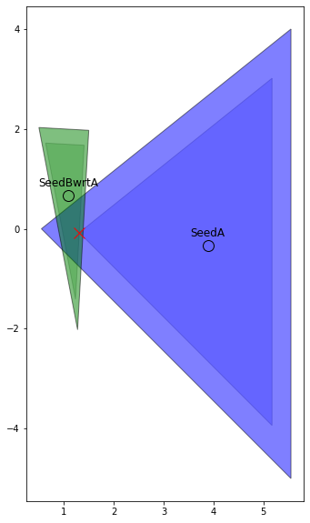
This is probably a bit complex but we can check this plotting for the sub-objects and see that the result makes sense. The one thing to note here is that since we are going to be checking for no interference we are not worried about the expansion, so if the value of the result gdDistance is larger than 1 then we set the value to 0.
fig, ax = plt.subplots(figsize=(10, 10))

shapeA = Polygon(gdVertA)
shapeAs = scale(shapeA, fscale, fscale, origin=tuple(seed_a))

polyA = PolygonPatch(shapeA, fc="b", alpha=0.5)

shapeB = Polygon(gdVertBwrtA)
shapeBs = scale(shapeB, fscale, fscale, origin=tuple(seed_b))

polyBwrtA = PolygonPatch(shapeB, fc="g", alpha=0.5)

ax.add_patch(PolygonPatch(shapeAs, fc="b", alpha=0.2))
ax.add_patch(PolygonPatch(shapeBs, fc="g", alpha=0.2))

ax.add_patch(polyA)
ax.add_patch(polyBwrtA)

ax.plot(gdSeedBwrtA[0], gdSeedBwrtA[1], 'ok', markersize=12,  mfc='none')

ax.plot(gdSeedA[0], gdSeedA[1], 'ok', markersize=12, mfc='none')

ax.annotate('SeedA', tuple(gdSeedA), textcoords="offset points",
            ha='center', xytext=(0, 10), fontsize=12)

ax.annotate('SeedBwrtA', tuple(gdSeedBwrtA), textcoords="offset points",
            ha='center', xytext=(0, 10), fontsize=12)

ax.plot(res.x[0], res.x[1], 'xr', mfc='none', markersize=12)

ax.set_aspect('equal', 'box')
Since we want to determine a measure of how much penetration there is between all the sub objects then our total value is just the sum of all resulting growth distances.
def poly_growth_fun(subObjsA, subObjsB,conf, verbose=False):
  gds=[]
  bad_res=[]
  for An,subObjA in enumerate(subObjsA):
    for Bn, subObjB in enumerate(subObjsB):
      gd, res = growth_distance(subObjA, subObjB, conf)[:2]
      if verbose:
        print('A{}-B{} | Status: {}, \
        Success: {}, \
        Value: {}'.format(An, Bn, res.status, res.success, res.fun))
      if res.status==2:
        bad_res.append([An, Bn])
        raise
      else:
        gds.append(gd)
  return np.array(gds).sum()
Checking Feasibility
Now that we can measure both the distance from feature to feature and the penetration we can crate a funtion that combines those two values.
def opt_fun(cs, subObjsA, subObjsB, conf, verbose=False):
  Ve_value=valueVE(cs, conf)
  Gf_value=poly_growth_fun(subObjsA, subObjsB, conf)
  if verbose:
    print('V_E value {}, Growth_Value {}'.format(Ve_value, Gf_value))
  return Ve_value+Gf_value
Genetic Algorithm
Since solving the equations to obtain a configuration that is has contact between the objects and also not penetrating is very complex (and not feasible once we get into more complex/ 3d objects). We instead will optimize the configuration in the possible space such that the result is equal to 0. If we can find a configuration then the contact state is possible.
To perform this optimization we use a genetic algorithm that basically emulates the evolution by converting the attempted values \( x \) into a chromosome and performing evolutionary changes to it based on a fitness function. Basically the xs that result in a higher function have a higher chance to reproduce. We keep some variety with mutations to help us avoid local minimums.
For us each individual in our population is an attempted configuration in the space.
Back in the day I used MATLAB's ga (and at some point GAlib). However that is not open source, there are a couple of options for python, most well know DEAP. However I decided to use Pygad to check it out.
Pygad is different from MATLAB's ga in that it maximizes the fitness rather
The first step in a genetic algorithm is to define a fitness function. For our case we just do the following.
def fitness_func(conf, index):
  fval=opt_fun(current_cs, subObjsA, subObjsB, conf)+thresh
  fitness=1/np.abs(fval)
  return fitness
Notice that we are minimizing fval and because of that we take 1/fval.
Quick thing: In both our calculations of distances h1, h2 and gd we defined 0 as a value less than a threshold. The reason is that dividing by 0 in numpy can cause the genetic algo to not work properly
Then we defined the bounds of our space of possible configurations
gene_space=[]
for l,u in zip(lb, ub):
  gene_space.append({'low':l, 'high':u})
Finally to show our work we create a callback after each generation.
def on_generation(ga):
    print("Generation", ga.generations_completed)
    print(ga.best_solution()[1])
Finally we define our instance
global current_cs
# we cant pass aditional parameters to the function, so we pass the
# contact state into a global variable, in this case we chose the last one
current_cs = ContactStates[-1]

ga_instance = pygad.GA(num_generations=100,
                       sol_per_pop=30,
                       num_genes=3,
                       num_parents_mating=5,
                       gene_type=np.float32,
                       gene_space=gene_space,
                       fitness_func=fitness_func,
                       crossover_probability=0.4,
                       mutation_type="random",
                       mutation_probability=0.6,
                       on_generation=on_generation,
                       allow_duplicate_genes=False,
                       stop_criteria=["reach_{}".format((1/thresh)-1), "saturate_50"])
We tweak each parameter depending on performance, the important ones are as follows.
num_generationsnumber of generations, this can be played around with but the more generations the longer our optimization could takesol_per_pothe number of individuals per generationnum_geneshow many chromosomes (values) exist in each individual, in our case this is 3 since we have configurations as \( x, y, \theta \).gene_typeI defined this as anp.float32since I don't have any interest in that many decimals and this reduces the calculation time.gene_typethe previous define bounds on created individualsstop_criteriatells the optimization when to end. In our case we set it so that is ends if the value is(1/thresh) -1which is basically 0 for our purposes and if there is no change after 50 generations (this can be played around).
Because of the way we setup these functions there will be a siginificant jump once we actually get zero.
Generation 1
25.727673594793036
Generation 2
25.727673594793036
Generation 3
59.70383773709654
Generation 4
59.70383773709654
Generation 5
59.70383773709654
Generation 6
59.70383773709654
Generation 7
59.70383773709654
Generation 8
59.70383773709654
Generation 9
59.70383773709654
Generation 10
1000.0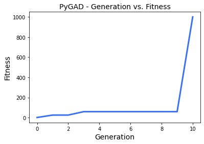
From that result we can see that the Contact State[-1] is actually possible.
We can take a look at how the assembly looks for a given contact state.
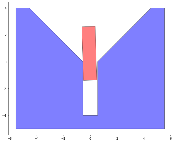
So we can determine the feasibility by doing checking the end fitness and seeing if its less than the thresh or not.
fit_res=ga_res[1]
if fit_res<=1/thresh:
  feasibility=True
  print('Contact State {} is feasable'.format(current_cs['ID']))
else:
  feasability=False
  print('Contact State {} is NOT feasable'.format(current_cs['ID']))
We can now iterate thru our list of primitive contact states and determine which ones are actually possible in the configuration space.
Conclusion
Well that was quite a lot of work and frankly gave me flashbacks to many sleepless nights. In all honesty Pygad is a great tool but I did miss the sleekness of Matlab's ga. The next step (and what I had to do for my thesis work) is to parallelize the code, and perhaps that is where a big improvement can be made, since there has been significant advancement in those areas in the last decade.
The next steps require a lot more work that I might undertake at a different time. It requires determining the extremal positions of each contact state (including E-V, and the dual conbination of then E-V | V-E, V-E | E-V and and theoretically V-E | V-E for shorter parts.
Finally to actually design the flexible manipulator (or Admittance Matrix) we need to define a bunch of constraints in screw notation related to contact wrenches and optimizing on that. This part would be a stretch to do since frankly I get stressed out just thinking about remembering how to work in screw notation.
Anyways a the jupyter notebook with all of this can be found in my github.